Before a computer can help with electrolytes or batteries, it has to look at a molecule drawn in a paper and know who it is. I post-trained vision-language models to read real paper figures, built VERDICT to check their answers by letting four independent readers vote (and abstain), tried a rotation-aware recognizer, and then turned the recognized molecules into vectors and a multimodal database. The best model read 59.8% of 331 real journal figures exactly, on par with a strong established reader, and agreement between readers separated right answers from wrong ones with an AUROC of 0.916.
Only people can read the drawings
The problem I started from is that a lot of chemistry is locked inside drawings that only people can read. Molecules are where this series starts, because electrolytes are mixtures of molecules and batteries are built around electrolytes, so everything later depends on this first step.
Pixels, not FEC
Papers and patents are full of molecule figures. A chemist glances at one and says “ah, FEC.” A computer sees pixels. As long as that’s the case, every molecule in the literature has to be found by someone squinting at a PDF. If you want to search by structure, or pull every molecule a paper tested into a database, you need recognition that a computer can do at high throughput.
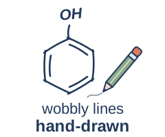
And not only for neat drawings: people sketch molecules by hand, too. A recognizer that only reads textbook-perfect drawings is reading half the library.
Same molecule, many drawing styles
The catch is that papers draw the same molecule in wildly different styles: thin double bonds, atom labels the size of a dust mite, wedge bonds, scans that look like they went through a fax machine twice.
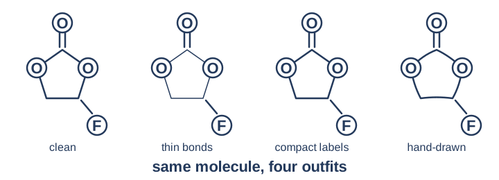
The way I thought about it was simple: atom is atom, bond is bond. However a paper draws FEC, it’s the same atoms joined by the same bonds, and that’s all recognition should care about. A model trained mostly on one drawing style doesn’t work that way, though. Show it the same molecule in an unfamiliar style and it can easily get it wrong.
Synthetic data is endless, real data is the exam
To teach it, I had two kinds of training data. Synthetic drawings are free and endless: chemistry software (RDKit, RDKit-coordgen, Indigo, RanDepict) can render any molecule in many styles. Real drawings are scarcer and messier: USPTO patent figures, UOB, and DECIMER-HDM, a set of hand-drawn molecules.
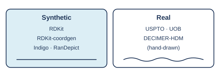
Here’s the trap. Because synthetic drawings are endless, it’s easy to train a model that looks amazing on them. But the real bottleneck wasn’t the amount of data. It was distribution shift: the gap between tidy rendered training images and messy real paper figures. A model can ace the rendered exam and still flunk the real world. Most of my summer on molecules went into three attempts at closing that gap.
Post-training a vision-language model
My first attempt was to take a general vision-language model and post-train it to read molecule drawings, and it worked about as well as a strong established reader.
How a VLM reads a drawing
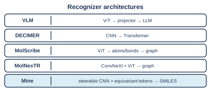
A vision-language model (VLM) looks at an image and writes text about it. Inside, an image encoder (a ViT) chops the picture into patches and turns them into vectors, a small projector translates those vectors into the language model’s space, and the language model writes the answer. Here the answer is a SMILES string, a line of text that spells out the molecule atom by atom.
Three base models, six data mixtures
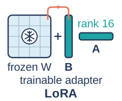 Supervised fine-tuning with LoRA
I compared three public base models, GLM-4.1V-9B, InternVL3-8B and Qwen2.5-VL-7B, across six mixtures of real and synthetic images, using supervised fine-tuning (SFT) with LoRA. LoRA is the “don’t renovate the whole house, just add a small extension” approach: instead of changing every weight in a big model, you learn small low-rank updates next to the frozen weights.
Deep dive: training recipe and keeping the test honest
My recipe was LoRA rank 16, BF16 numbers, small batches, activation checkpointing (recompute some things instead of storing them, to save memory), and selective adaptation of the vision part. Unglamorous, but it fits on the hardware.
To keep myself honest, I split the data by molecule identity and excluded 55,267 benchmark molecules (by InChIKey, a fingerprint of chemical identity) from training, so the model couldn’t just memorize the test. I scored three things: whether the SMILES is valid, whether it’s an exact match, and, for wrong answers, how close they are (Tanimoto similarity of fingerprints).
The winner was GLM trained with 70% real images, at 59.8% exact structure on 331 figures from ACS journals. That’s statistically comparable to MolScribe (58.3%), a strong established reader. I wrote more about the real-versus-synthetic story in the paper.
The DPO detour
Then I got ambitious and tried DPO, a preference-tuning method that teaches a model to prefer good answers over bad ones. The training curves were gorgeous: loss dropped from 0.69 to 0.19, and preference accuracy hit 90–97%. Exact match on the molecules it actually generated was 0–2%. The model had learned to win the preference game, not to read molecules. A second attempt improved validity but still landed at roughly half the accuracy of plain SFT, so I kept SFT.
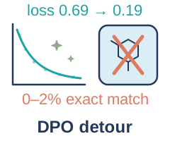
Pretty loss, wrong molecules. What I took from it is that a pretty training score can miss the scientific goal.
VERDICT: four readers and permission to say “I don’t know”
Once the model could read, the next problem was trust. My plan was to run it over many more real drawings from papers and use its answers as new training labels. But on a real page there is no answer key, so even when the model was confident, I had no direct way to tell whether it was right. Working out how to check it became VERDICT.
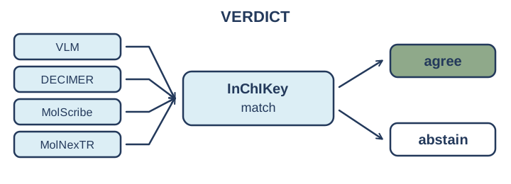
VERDICT
Instead of trusting one model, VERDICT asks four: my fine-tuned VLM plus three open-source readers, DECIMER, MolScribe and MolNexTR, each built differently. It compares their answers by chemical identity (InChIKey), not raw strings, because two different SMILES strings can describe the same molecule. It keeps the disagreements and where each answer came from, and it is allowed to abstain.
A 3-to-1 split, kept in the open
A real example from my notes: on one FEC image, three readers got it right and one read an F as an I. VERDICT didn’t quietly pick a winner; it kept the 3-to-1 split and showed it.
Agreement is a good signal for correctness
Agreement separates right from wrong answers with an AUROC of about 0.916, versus 0.547 for checking how similar a redrawn image looks to the original, which is barely better than a coin flip. I ran VERDICT over about 38K real crops from papers and fed the labels with 3-of-4 agreement back into training. The retraining gains were mixed, so I report data quality and model improvement separately. The whole point of VERDICT is that I didn’t want to take any single model’s word for how accurate it was.
Rotation yes, mirror no
My third attempt was to build one piece of chemist common sense straight into the architecture: a rotated drawing is the same molecule. Turn a drawing 30° and nothing about the chemistry changes, but an ordinary CNN has to learn that from data, usually by training on randomly rotated copies. I wanted the model to know it by construction, so it can’t forget. That’s my public research repo, Ouroboros.
The trap is in your hands
Your left and right hands are mirror images: same fingers, same knuckles, yet a left glove won’t fit your right hand. Many molecules come in left- and right-handed versions like this, which chemists call chirality. The two look nearly identical on paper but can behave drastically differently, in a body or in a battery. In drawings, handedness is carried by wedge and dash bonds, the little triangles that say “this bond points toward you” or “away from you.”
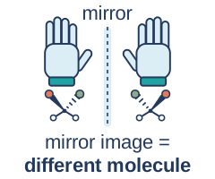
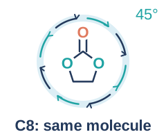
So the model should give the same answer when the drawing is rotated, but it must not treat the mirror image as the same molecule. In equivariance jargon, the full group of flat rotations and reflections is called E(2); I deliberately kept only the rotations, a rotation group C_N with no flips (escnn’s rot2dOnR2). In the repo’s mirror test, all 200 of 200 mirrored renderings were labeled as the enantiomer, the mirror-partner molecule, not the original. Left glove, correctly identified.
How the model keeps rotation
The image encoder is a steerable CNN over C8, eight discrete rotations 45° apart, and its tokens keep track of direction instead of throwing it away.
Deep dive: steerable filters and position × direction tokens
The steerable CNN’s filters follow known rotation rules, so rotating the image transforms the features in a predictable way instead of scrambling them. That’s exact for 90° rotations, where pixels land back on the pixel grid, and approximate for other angles, because pixels are square and the world isn’t.
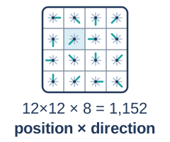
The usual move after the encoder would be to squash the features into one token per patch, which throws the direction information away. I kept “position × direction” tokens instead: on a 12×12 grid with 8 directions, that’s 1,152 tokens. Attention between tokens only sees relative position and relative direction, with the relative position written in the asking token’s own direction frame. Rotate the whole picture and the tokens just get relabeled consistently, so nothing about the answer changes. After attention, I average over directions and hand the result to the SMILES decoder.
Three arms
To test it, the repo has three arms: A, an ordinary CNN; B, the same CNN trained on randomly rotated copies; and C, the C8 steerable CNN plus the rotation-aware token mixer. All three trained on 200,000 synthetic examples.
The honest label is that this is a synthetic-data, single-seed research preview. Accuracy on real documents isn’t established yet, and stereochemistry (those wedges again) is still a source of errors.
From a name to a vector
Recognizing a molecule gives you its identity, but a model needs a vector it can compute with.
Three ways to describe a molecule
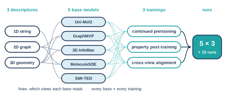
A molecule can be described in at least three ways. A 1D string is SMILES, a fingerprint or a text description. 2D topology is the graph: which atoms connect to which, and how big the molecule is. 3D geometry is where the atoms actually sit in space, a conformer. It’s like describing a friend by their name, their family tree, or a photo.
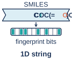
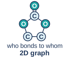
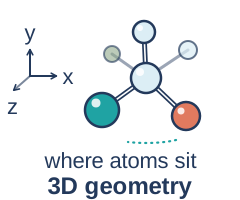
Getting from the drawing to the photo is a pipeline: 2D image → SMILES → 3D conformer → energies and forces, computed with machine-learned potentials like MACE and UMA.
Five base models
Rather than invent a new model for the vectors, I started from five public base models, each of which learned about molecules in its own way.
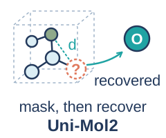 Uni-Mol2
Hides some atoms and learns to recover them from atoms plus their positions in space.
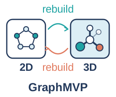 GraphMVP
Makes the 2D graph and the 3D conformer reconstruct each other.
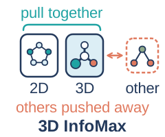 3D InfoMax
Pulls a molecule’s graph and 3D views together and pushes different molecules apart.
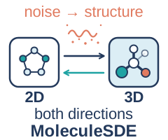 MoleculeSDE
Generates 3D from 2D and back, plus the same pull-together trick.
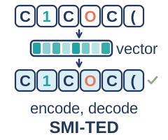 SMI-TED
Reads SMILES and learns to rebuild the token sequence.
Three ways to adapt them
Then I adapted each of them to my data in three ways.
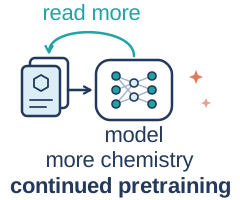 Continued pretraining
Keeps each model’s own self-supervised objective and simply runs it on my molecules.
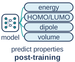 Property post-training
Teaches properties I care about: energy, HOMO/LUMO, dipole, volume and electrostatic potential, and for formulations, conductivity, density and viscosity.
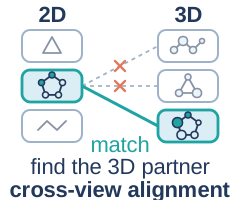 Cross-view alignment
Uses InfoNCE, where a 2D view has to pick out its own 3D partner from a crowd of other molecules in the batch.
Five bases times three training types is 15 adaptation runs. The result was refreshingly untidy: no single training type was best for every task. Alignment helped views find each other; property training improved some properties while weakening cross-view matching. You get what you train for, and sometimes you pay for it elsewhere.
What the extra views really added
With fifteen runs on the table, I wanted an honest answer to a simple question: did the extra views, especially 3D, bring new information, or just more numbers? Most of this is from my notes and experiments; where I’m thinking out loud instead of reporting a result, I’ll say so.
The 2D graph says which atoms are connected; 3D says how they’re arranged in space. A flexible molecule can keep the same connections and take different shapes, so 3D can add something new. But it can also mostly repeat what 2D already implies, like size and composition. In a scaffold-held-out comparison, real 3D added to 2D cut electronic-energy error by about 18.2% and volume error by about 49.4%. That’s one controlled comparison, not a law for every model and property.
Finding a molecule’s other view and predicting its properties also turned out to be different abilities. Among 5,000 candidates, aligned representations found the matching other view first (R@1) about 0.760 of the time, versus 0.0756 for the base representations and 0.0074 after property training. Property training nearly erased matching.
Deep dive: the controls, and why copying isn't understanding
To tell new information from repetition, I compared composition only, 2D, 3D, 2D+3D, and a sneaky control: 2D plus shuffled 3D, where each molecule gets another molecule’s geometry. If the shuffled version helps just as much, the “gain” is a shortcut or just extra dimensions. I also used scaffold-held-out splits, frozen-representation probes, perturbed coordinates and removed inputs.
Copying turned out to be different from understanding, too. A SMILES-only “student” trained to copy a 3D “teacher” matched the teacher’s vectors closely, yet some experimental conductivity tasks didn’t improve. So I tried a branch that keeps the original 2D information while learning geometry. A distance-only 3D branch, which reads distances between atoms but not which elements they are, responds to distance changes but can’t tell every chemical identity, or handedness, apart. And randomly dropping inputs during training mainly helped when 2D was missing at random, not when a whole chemical class was missing or when extrapolating to low temperature.
My conclusion from all of this is to test view matching, teacher matching and property prediction as separate abilities, and to judge an extra data type by whether it helps the actual scientific task, measured against strong single-input models, simple fusion, correct pairs and shuffled pairs.
Molecules become ingredients
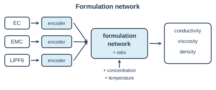
Those molecule vectors then become ingredients. A formulation network takes one vector per molecule, plus mixing ratios, salt concentration and temperature, and predicts how the mixture behaves. That’s a first taste of Part 2.
A truly multimodal database
All of this pays off in one place: once recognition is reliable, every molecule pulled from a paper becomes an entry in a truly multimodal database.
One molecule, many ways to know it
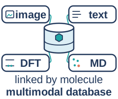
It helped me to draw how the views relate. The image is how a paper drew the molecule. The text is what the paper says about it. The 1D/2D/3D structure says who is bonded to whom and where the atoms sit. DFT properties are electronic: energies, HOMO/LUMO, how readily it gets reduced. MD properties are collective liquid behavior: solvation, density, diffusion, transport.
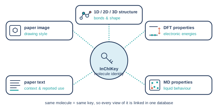
The molecule’s identity, the InChIKey that VERDICT checks, is the shared key that links all of them, and alignment (InfoNCE) places the views in one shared space. Some information overlaps: 2D and 3D both know composition and size. Some lives in only one view: geometry and stereo in 3D, context and reported use (solvent, salt or additive?) in the text, and collective behavior only in MD.
Why not just text?
This next bit is framing rather than a result: a text-only language model sees only what someone wrote down about a molecule, not its geometry or how it moves, and a lot of chemistry never gets written down as sentences. My non-text inputs over the summer were molecular images, atom graphs, 3D coordinates, MD trajectories, simulation-state vectors and experimental numbers. There are several ways to hand them to a model: write the numbers into a prompt as text, use graph encoders, use time or sequence models, project them into an LLM as “soft tokens,” or use retrieval and evidence tools. VERDICT is a verifier of the last kind, built on agreement between independent readers and chemical identity.

I judge each route by whether it helps the target task, and I keep asking what useful information survives compression. Squeezing 5,000 frames into one vector is great, unless the squeeze throws away the physics; a small representation is useless if it lost the essential part. That’s also why my cell assistant in Part 3 shows measured, computed and predicted values separately, along with which records a conclusion used.
Retrieval, starting from a picture
What I was building was scientific multimodal retrieval and alignment: SMILES and 2D graphs, the image from the paper, the paper’s description, 3D geometry, and non-text values from multi-scale simulations, all linked by the same molecule. Image ↔ text ↔ 3D geometry ↔ DFT ↔ MD.
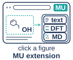
People use it through the MU product and a Chrome extension, and the point is fast retrieval starting from a picture.
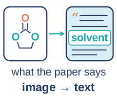 Image → text
From a molecule image, jump to the paper’s own description of it.
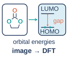 Image → DFT
Properties computed by DFT, such as its electronic properties and how readily it gets reduced.
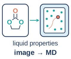 Image → MD
Properties computed by MD, such as solvation, density, diffusion and transport.
Notice the last one. MD properties aren’t about a molecule on its own; they’re about what it does in a crowd.
What this got us
By the end of Part 1, a molecule in a paper was no longer just pixels: it had a checked identity, 1D/2D/3D vectors from fifteen adaptation runs, and computed DFT and MD properties, all linked in one database. In hindsight this was the first layer of something bigger, recognize and represent, with a verifier attached. Part 2 takes these molecules and their computed properties, mixes them into electrolytes, and asks the much harder question of how they move.