The electrolyte formulations from Part 2 go into real cells here, and the question becomes the one a battery company actually cares about: if I change the recipe, what changes in the battery? Starting from 252 additive-centered formulations, I stacked the molecule and electrolyte representations from Parts 1 and 2 into a cell representation, built a ladder of multiscale simulations around the real recipes, aligned the scales, trained an aging world model that learns how a cell evolves instead of guessing one lifetime number, and wrapped it all in a cell co-scientist. The clearest finding was that test conditions are the glue between scales: removing them collapsed a key cross-scale link score from 0.327 to 0.066.
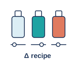
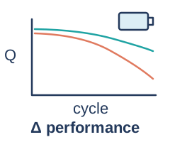
Δrecipe → Δperformance
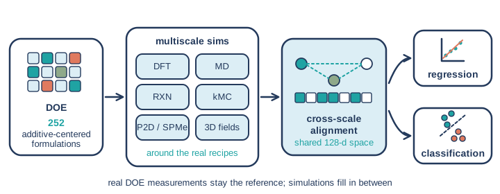
My starting point was a real, specific problem: a design of experiments (DOE) of 252 cell formulations built around additives, and a lot of questions about it.
Change the recipe, watch the battery
Within each comparison the electrodes were held fixed and the additives changed, so any change in performance can be pinned on the recipe. The question is simple to say: change the recipe, and what changes in capacity retention, cycle life, resistance and rate? In practice that meant looking at cycling, storage, charging and rate tests.
Slow bakes, plenty of compute
It’s a bit like baking. Swap one ingredient and the cake might rise higher, or collapse, or taste fine today and go stale next month. The annoying part is that each real bake for a battery is slow and expensive, and there was no budget for repeated new rounds of experiments. Compute, on the other hand, was available. So the plan was to use compute to fill in around the real data, while real measurements stay the reference. Simulations get to advise; they don’t get to overrule.
A cell is a stack of representations
The idea that unlocked this part is that nothing from Parts 1 and 2 had to be thrown away. Both were, at heart, representation learning.
Reuse, don’t restart
Part 1 turned every molecule into vectors from its 1D, 2D and 3D views. Part 2 turned every electrolyte into 128 numbers in a shared latent space, learned from recipes, snapshots and trajectories. A battery cell can be represented by stacking those learned pieces: the molecule representations for each component, the electrolyte latent for the mixture, and the cell’s own design and operating conditions on top.
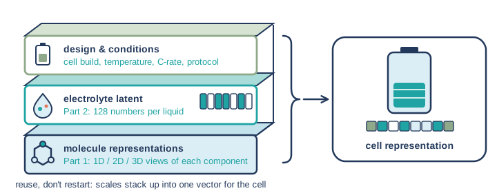
Molecules make up electrolytes and electrolytes go into cells, and here the representations follow the same path.
Simulations around the real recipes, lined up
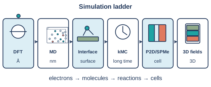
A stack of representations needs something to learn from, and 252 formulations is not a lot, so I spent about a month building a high-throughput ladder of high-fidelity simulations around the DOE itself: around its real recipes and its real test protocols, not around made-up chemistry. No single simulation covers everything from electrons to a whole cell heating up, so each rung hands something to the next.
Six rungs
Here are the six rungs, from the smallest scale to the largest.
 1. DFT
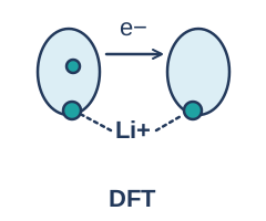
Electrons and local chemistry: whether an additive can be reduced, who coordinates around the ion, and how much energy it takes for a molecule to decompose. That local chemistry is the starting point for the liquid.
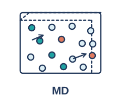 2. MD
How molecules organize and move in the liquid: solvation, aggregation, diffusion and conductivity. This is the PFF from Part 2, and it supplies what arrives at the electrode.
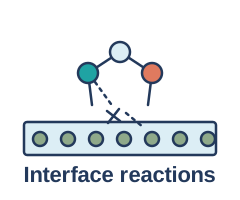 3. Interface reactions
How molecules may change near the electrode, the battery’s busiest border crossing, where bonds break and form. I explored these with a learned force model, and the events it finds become the moves for the next rung.
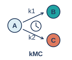 4. kMC
Kinetic Monte Carlo thinks in states, events and rates, like a board game where each move happens with some probability per unit time, to ask what happens next over long times. In my setup, kMC sits inside the cell model, the next rung.
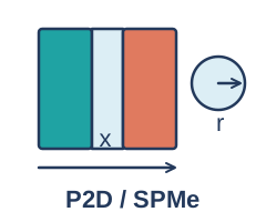 5. P2D / SPMe
The whole cell’s transport and reactions: voltage, capacity and aging. P2D resolves what happens through the electrode’s thickness and inside its particles; SPMe is its simpler, cheaper cousin for when you need many runs fast. Both treat the cell as one stack.
 6. 3D fields
Temperature and stress varying across the cell. I ran 3,331 electrothermal simulations linked to DOE records, using the recorded protocols, with stated assumptions about geometry and thermal inputs.
Deep dive: what the kMC rung did and didn't show
When I compressed MD transport into 12 states, the model’s held-out transition NLL was 1.612 versus 2.273 for an independent-state baseline (lower is better). Full SEI growth was not validated, so I’m not claiming it.
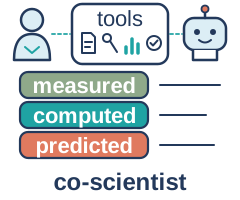
Every calculation keeps its recipe, conditions, source and a fidelity label: measured, calculated or predicted. Mixing those up is how you end up trusting a simulation more than the experiment it was supposed to explain.
Lining up the scales
With simulations at every scale, the next step was to connect them, the same way Part 2 connected recipes, frames and motion. Each input got its own encoder, mapped into a shared 128-d space. Then I learned links between neighboring scales: DFT ↔ molecules, molecules ↔ formulations, formulations + conditions ↔ MD, MD + conditions ↔ cells, cells + conditions ↔ DOE, plus links for the interface. The loss was a multi-positive InfoNCE, a fancy way of saying “pull together everything that belongs to the same experiment, push apart everything that doesn’t,” along with predicting the next scale’s vector from the current one.
To keep myself honest I trained four versions, three seeds each: the full model, no conditions, shuffled pairs, and no extra linking loss. Two findings stood out.
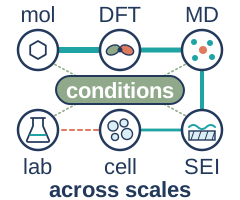
Conditions are the glue. Temperature, C-rate and protocol are what connect the scales: removing them collapsed the MD-to-electrode link score from 0.327 to 0.066. Without knowing how a battery was tested, the scales stop recognizing each other. Correct pairs also scored much better than shuffled ones, so the links are real.
The second finding is that molecules don’t get you to a battery just via alignment. Matching a molecule’s identity across views could be strong while the links to the real DOE stayed weaker.
Property heads
On top of the shared space sit regression and classification heads for property prediction. With chemistry inputs only, the normalized error (MAE across DOE targets) fell from 0.3341 to 0.2849 using modality dropout, which means randomly hiding inputs during training so the model learns to cope when some are missing. It cost a little when every input was available (0.2442 → 0.2542), a trade I’ll happily take. And the uncertainty was overconfident: nominal 90% intervals covered only about 68–78%, so the stated uncertainty needs widening before anyone relies on it.
An aging world model
The heads still predict a target as one number, and that’s the habit this section breaks: the goal shifted from predicting lifetime to learning the whole evolution process, how the cell’s state evolves under its design and its conditions.
From one number to the whole story
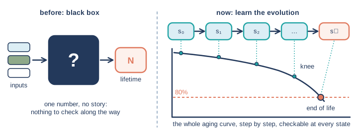
The usual black box takes the recipe in and gives one number out (“lifetime: N cycles”). It gives you nothing to check along the way, and when it’s wrong, it can’t tell you why.
Simulations as the practice data
To learn a process you need to watch it happen many times, and real experiments are few and slow. Simulations, on the other hand, give dense, state-by-state trajectories under many designs and conditions. So I ran a large number of P2D and 3D aging simulations: expensive, long DFN (full P2D) runs for some cases and cheaper, short SPMe runs for many more, screening early and recording why each run stopped. The 3D layer added 100,000 electrothermal entries and 200,000 chemical-mechanical results. The DOE stays the real-cell reference throughout.
How it works
 Aging world model
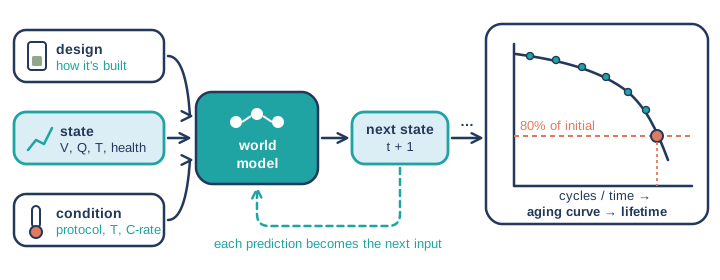
Given the cell’s design, its current state (voltage, capacity, temperature, aging variables, state of health) and the condition (how it’s being used: protocol, temperature, C-rate), it predicts the next state. Then it rolls out: each prediction becomes the next input, step by step, into a full aging curve, and the lifetime is read off where the curve hits an endpoint, for example 80% of initial capacity. The same machinery covers calendar aging (sitting on a shelf) and cycle aging (being used).
It’s like predicting tomorrow’s weather, then using that forecast to predict the day after.
I compared 41 architectures on an early dataset of 6,258 simulated sequences × 140 steps, and the learned world model beat a direct MLP baseline on simulated sequences. My historical summary recorded roughly 24–27% lower error. I haven’t yet traced every one of those numbers back to its fold and target, and to be very clear, it is a lower prediction error on simulations, not an increase in anyone’s real cycle life.
Four checks
Next-step accuracy
Does one step forward land in the right place?
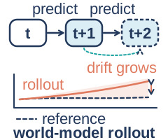
Long-run drift
Harsh, because each output becomes the next input and small errors snowball.
Direction of change
Does the curve move the right way when you swap an additive or a condition?
Agreement with experiments
Does it match real cells, not just the simulator?
The honest gap is that a model that learns the simulator very well can also inherit the simulator’s mistakes. How well it learns the simulations and how well it matches real cells are separate questions.
Knowledge emergence, carefully
Here’s the part that got me most excited, and I want to be careful with it. Because the model learns the process instead of memorizing endpoints, I started to see it pick up physically sensible chemistry and battery behavior that nobody spelled out for it, which is what I’d call knowledge emergence.

That’s my observation and interpretation, not a measured result. What I can point to is how it gets checked: rollouts are inspected for unphysical behavior in capacity, temperature and concentration at different horizons, held-out operating conditions test whether the model responds in the right direction, and the direction-of-change check is one of the four tests above. I’m not claiming it discovered anything specific like SEI growth or lithium plating. Confirming emergence rigorously is ongoing work, and probably my favorite open question from the summer.
Checking against real cells
Simulations are the practice field, not the match, so the last scientific step was to hold the models up against the DOE.
The VC plot twist
My favorite plot twist came from one additive, VC. In matched DOE comparisons it hurt cycle life in one cell design and helped in another. Same ingredient, opposite story. A physics model built on a fixed VC-SEI hypothesis reproduced some of the sign changes, but not the full direction and size of the effect. That sounds like a failure, but it’s the most useful kind of result: it turns the hypothesis into a candidate mechanism with a concrete next test.
Calibration, not self-grading
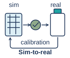
A rule I try hard to follow: don’t tune a model on the DOE and then hold up the same DOE as validation. That’s grading your own homework with the answer key taped to the back.
The bridge between simulation and reality is calibration against real experiments, and the sim-to-real calibration supported 24 targets. Everything else stays labeled for what it is: simulated until a real cell says otherwise.
A cell co-scientist
The last piece was the same move as at the end of Part 2, one scale up: hand everything to a co-scientist that can reason over it. This time the inputs come from every level.
Inputs from every level
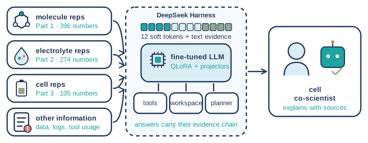
In the early version, each record carried numbers from all three parts, 775 in all.
396 molecular
Molecular features from Part 1.
274 electrolyte
Electrolyte features from Part 2.
105 cell
Cell features from this part.
Each group goes through its own small projector into 4 “soft tokens,” and the 12 soft prefix tokens sit in front of the text, with missing inputs masked. Tokenization is chemistry-aware: common molecule names are kept as single tokens, with markers for chemistry and scale, so names get read as chemistry rather than letter soup.
Deep dive: text evidence, explanation examples and the training split
Next to the numbers goes text evidence: the recipe, the conditions, measured and simulated results, and where each came from. I also built explanation examples from evidence packages: a teacher model writes the explanation, and a critic plus fixed rules check it. A first pilot had 300 examples covering complete, missing, novel and conflicting evidence. On top of that come the data, the simulation logs and the tool-usage records. Held-out experimental answers stayed out of training, forward prediction can’t see the target value, and the split is by recipe. The fine-tuning itself is LoRA (QLoRA) on the LLM, trained together with the scientific projectors.
The harness and the split between two models
 Cell co-scientist
The harness is DeepSeek Harness, connected to battery tools: cell prediction, recipe suggestions, similar experiments, cross-scale explanations, multiscale evidence, and formulation comparison, plus a call to the trained specialist that attaches the record’s evidence chain. A workspace keeps the conversation, the explanations and the tool history.
The work is split between two models: a larger LLM handles planning and tool calls, and the fine-tuned compact open-weight LLM acts as the scientific specialist. Its training data didn’t include tool-call trajectories, and I learned that good scientific answers don’t automatically give you reliable tool use.
What it can do
It connects recipes, conditions, simulated states and measurements; explains an answer with sources; compares candidate formulations; suggests recipes; finds similar experiments; and says what evidence is missing and what the next useful calculation would be. The interface shows the explanation, the tool calls, the returned results and the record IDs, and it marks every piece of evidence as measured, computed, predicted, missing or rejected. If you’ve read this far, you know why that matters to me.
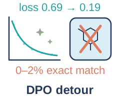
To be honest about where it stands: in the demo, prediction and inverse design still used DOE retrieval and ranking of measured recipes, and connecting the world model is further work. A first explanation-training pilot didn’t improve the combined score, so it stayed experimental. And the reasoning text it writes is an output to inspect, not proof of what happened inside the model.
A decision API for the small judgments
Watching the agent work gave me one more idea, which is design thinking rather than a measured result. A lot of what an agent does all day is small and repetitive: is this record relevant, which of these four candidates fits, how complete is this evidence on a five-level scale. Those steps need judgment or a score, not long reasoning, and they’re exactly where a general LLM can wander off and return something malformed.
Jev decision API
I’d route those steps through a decision API to Jev, TypeSafe AI’s decision model, released on 15 September 2026 as a “System One” decision model. Jev answers typed questions about a text or JSON state and only returns structured outputs: a Choice (pick from up to 255 options, with probabilities), a Score (a position on a rubric of 2 to 10 levels that you describe), or a yes/no probability.
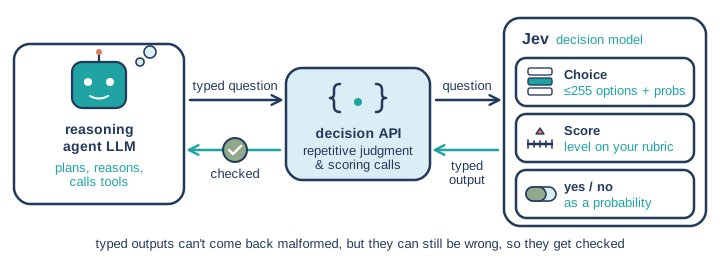
An independent evaluation reports 95–99% accuracy on several classification benchmarks and well-calibrated choice probabilities. Its “can’t hallucinate” guarantee is about format: the output always matches the declared schema, so no invented options and no parse errors. It isn’t a guarantee of correctness, and it can still pick a valid but wrong answer, which is why those steps still get checked. The point of the split is that the small judgments never come back malformed and come with calibrated probabilities, and the reasoning LLM is freed to do what it’s good at, which should make the whole agent stronger.
I’d like to say this is now a finished method of my own: represent, align, predict, then a co-scientist with a decision API. Honestly, the field moves so fast that I spent the summer chasing the frontier and bolting new pieces on, and I expect to keep doing that. It’s a living method, and this is its current version.
What this got us
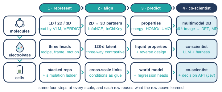
The summer followed the stuff itself. Molecules got recognized and represented (Part 1), mixed into electrolytes whose rulebook, movies and latent space I built (Part 2), and went into cells, where the representations stacked up, the scales got aligned, a world model learned how the whole thing ages, and a co-scientist learned to reason over all of it (Part 3). Looking back, the same pattern showed up at every scale: represent, align, predict, and hand it to a co-scientist.
I started from batteries and ended up with a method. Batteries were just where I happened to begin, and I think the pieces add up to a framework that should transfer to similar systems: complex material and chemical systems built as molecules, then mixtures or formulations, then devices, where the structure lives in non-text data like drawings, geometry, trajectories and simulations, the scales are linked by conditions, and experiments are scarce but simulation is possible. Through all of it, real experiments stayed the reference: simulations explore, models propose, measurements decide. Now if you’ll excuse me, I have a mechanism test to think about.