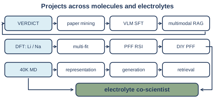
In Part 1 molecules got recognized and turned into vectors; here they get mixed into electrolytes, and the question becomes how they move. I extended a polarizable force field to 627+ molecules and 20+ anions, turned the failures of more than 50 of 80 versions into a self-improving fitting loop, and taught a model to read about 40,000 molecular-dynamics movies through three heads and one shared 128-number space. That space predicts conductivity with R² 0.976, and everything I learned along the way became training material for an electrolyte co-scientist.
How do molecules move in a liquid?
The question I worked on for this part was how molecules move in their micro-environment, and it starts with what an electrolyte actually is.
A crowded dance floor
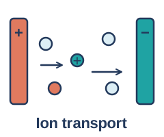
An electrolyte is the liquid inside a battery that ions swim through. The recipe is simple: salt + solvents + additives, and those are exactly the molecules from Part 1, now with jobs. The behavior is not simple. Zoom in and it’s a crowded dance floor: lithium ions grab solvent molecules as partners, anions try to cut in, and how fast everyone gets across the floor decides how well the battery charges and discharges.
A rulebook and a movie
To watch that dance on a computer you need two things. A force field is the rulebook for how atoms push and pull on each other. Molecular dynamics (MD) is playing the movie with that rulebook: put lots of molecules in a box, apply the rules, and watch. If the rulebook is wrong, the movie is fiction. Very confident, beautifully rendered fiction.
Writing a bigger rulebook
My first job was to grow the rulebook so that the molecules people actually want to try have rules to follow. The force field is polarizable (PFF), meaning electron clouds can squish in response to their neighbors, which matters a lot around small, charged ions like lithium. The goal was coverage: extend it to 627+ molecules and 20+ anions, for both lithium and sodium electrolytes.
Reference data from quantum chemistry
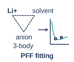
The reference data comes from quantum chemistry (DFT), and lots of it. Some clusters are binary: the ion with one partner. Some are ternary: a solvent and an anion competing for the same ion, like two people reaching for the last slice of pizza. Each pair or trio gets computed at many distances and orientations, so the rulebook sees close calls, near misses and awkward side-on approaches, not just the polite pose.
What actually got fit
What I fit was mainly the exp-6 cross terms, keeping the charges and the polarization background fixed. All the while I was debugging, learning electrolyte science on the fly, and studying the properties that came out. Three jobs at once, which is roughly how every internship works.
Deep dive: what exp-6 means
Exp-6 is the part of the rulebook that covers short-range repulsion (“personal space!”) and dispersion, the weak, sticky attraction between everything. The “exp” is an exponential wall that keeps atoms from overlapping; the “6” is a gentle pull that falls off with the sixth power of distance.
The liquid gets a vote
The hardest lesson of the summer was that a fit isn’t done when the cluster error is low; it’s done when the liquid behaves. Density, radial distribution functions (who stands next to whom), diffusion, conductivity and viscosity all have to come out sensible in MD. My ledger ended up indexing 80 distinct force-field versions, and more than 50 of them failed. Here are a few of my favorite ways to fail.
The penguin huddle
One fit looked great on the clusters. Errors low, curves lined up, very satisfying. Then I ran the liquid and it clumped: the ions huddled together like penguins in a blizzard. I traced it to one ether-oxygen interaction the fit had effectively broken. Restoring it cut the ion aggregation fraction from 0.811 to 0.282, and from 0.415 to 0.044 in a second system. Conductivity moved closer to experiment, though it was still too low. Progress, not victory.
The wall that rounded to zero
A tiny coefficient, 0.00170, got rounded to zero on its way into the simulation. The builder treated zero as “missing” and helpfully swapped a big repulsive wall for a small one, and MD failed. Now a check reads the final built parameters, not just the ones I meant to build.
The helium incident
Lone-pair virtual sites stored with the label “He” were passed to DFT as real helium atoms. That quietly affected 27 of 61 clusters. Nothing says summer internship like accidentally inventing noble-gas electrolyte chemistry. Now templates, masses and site types are checked before anything goes out.
The failure that was a success
A salt-free solvent control came out at a viscosity of about 2.1–2.4 mPa·s, which told me the solvent was fine and the problem lived in the salt model.
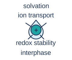
An electrolyte has many jobs, and a rulebook that only nails small clusters can still flunk all of them in the liquid. What I learned is that a low DFT fitting error doesn’t protect the liquid, and MD validation is part of parameter development, not a final demo.
PFF RSI: turning failures into checks
Fifty-odd failures is a lot of pain, but it’s also a lot of data, so I distilled them into a recursive self-improvement system, PFF RSI.
PFF RSI
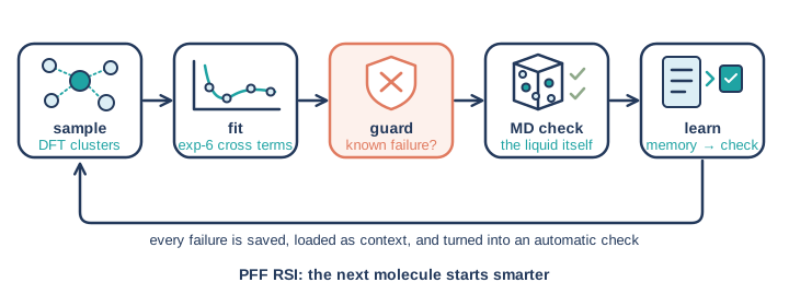
At its core it’s a simple cycle: fit the force field, validate in MD, record the failures, refine the next fit. When a brand-new molecule shows up, the loop runs on its own: sample, fit, guard, check in MD, learn, repeat.
Four layers under the cycle
Underneath the cycle, I built four layers.
Memory
A saved failure: the system, the version, what changed, what I expected versus what I measured, and what it cost, stored so it can be searched later by conditions, bad parameters, symptoms and useful checks.
Context
Loading the relevant failures before a new fit.
Code harness
Turning a failure into an automatic check, a new procedure written as code, so the same mistake gets caught by a machine instead of by me at 11 pm.
Weights
The fitted parameters that the whole loop keeps refining.
A new molecule arrives
When a brand-new molecule shows up, the loop samples a small starting set of clusters and expands only the channels that failed, fits, and checks. Parameters that match a known failure pattern get intercepted and sent to MD for a look before anyone uses them, so the wall that rounded to zero and the helium incident can’t sneak through twice. The honest caveat is that a fixed-budget test proving this memory actually makes research faster is still on my to-do list. It feels faster. Feelings aren’t data.
40,000 movies and three heads {#40000-movies-and-three-heads}
Once the rulebook works you can make movies, lots of them, and then you hit a new problem: none of it is text. Each trajectory is 5,000 frames, one every 4 picoseconds, for 20 nanoseconds in total. I ended up with about 40,000 trajectories, roughly 200 million frames.

You can’t paste a trajectory into a chatbot and ask how it felt. It’s coordinates, boxes and time, and the interesting part (who solvates whom, how ions hop) is spread across thousands of frames. So I asked whether a model could learn what a liquid is by watching, and squeeze each one into something small enough to search, compare and predict with.
Three views of the same liquid
I looked at the same liquid through three views, each with its own encoder, or “head.”
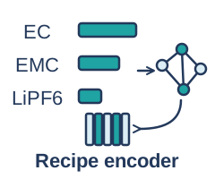 1. Recipe
What’s in the bottle: the components, their amounts, and conditions like temperature, turned into 128 numbers.
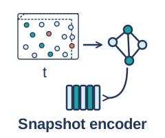 2. Snapshot
One frozen frame of 3D atoms. It’s my favorite, so it gets its own subsection below.
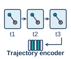 3. Trajectory
Motion over time: the 5,000 frames are split into 50 chunks of 100, so the model sees how things move, not just a pose.
All three are compressed into one shared 128-d latent space and trained with three-way contrastive alignment: views of the same liquid are pulled together, views of different liquids pushed apart. A recipe should find its own movie, and a snapshot should find its own recipe. That one space then does three jobs: retrieval, alignment between views, and property prediction.
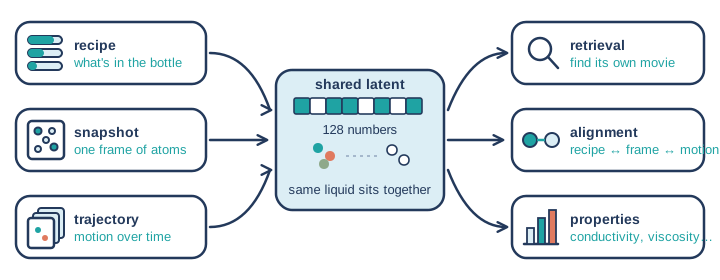
What the space can do
For retrieval, retrieval@10 (is the matching liquid in the top 10?) was 84.1% with the full representation versus 82.4% from the static snapshot alone, so a single frame already knows a lot. For conductivity, the model reached R² 0.976, close to a strong descriptor baseline, and adding trajectory features improved conductivity error in 18 of 21 held-out chemistry groups: motion helps, especially on chemistry the model hasn’t seen. Across the property heads, I got R² 0.906, 0.936 and 0.987 for conductivity, viscosity and solubility. The representation also carried over from lithium to sodium electrolytes with only a simple alignment step.
From there I took two more steps. Reverse design starts from the properties you want and looks for recipes that land there. I also tried trajectory generation, rolling the movie forward with GRU, TCN and causal-transformer models, though I won’t go into that here.
Inside the snapshot encoder
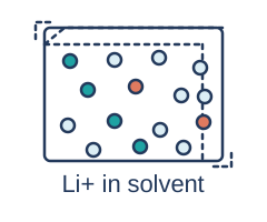 Snapshot encoder
The snapshot encoder is where the physics goes into the architecture, the same way rotation did in Part 1. Each frame becomes a periodic atom graph, and equivariant message passing turns it into 128 learned numbers plus 8 geometric ones, such as lithium coordination and ion contacts: 136 numbers per frame.
Every atom connects to neighbors within 6 Å, using the minimum-image rule across the box boundaries (the box wraps around like Pac-Man), and whole molecules are kept intact instead of getting sliced at the edge. Each atom then carries two kinds of luggage: plain numbers (scalars) and little arrows (vectors). Messages are built from distances and directions, so when you rotate the box, the arrows rotate right along with it and the final pooled numbers don’t change at all. The model doesn’t waste effort learning that a rotated liquid is the same liquid (the same “atom is atom” spirit as Part 1), while still keeping directional information like which way a solvent faces a lithium ion.
Deep dive: the unglamorous speedups
The unglamorous part made everything else possible. Neighbor search went from O(N²) to O(N): instead of every atom asking every other atom “are you close?”, each atom only checks its own neighborhood. Then I froze the encoder and cached about 192 million snapshots once, which took 395 H200 GPU-hours and a cache of about 52 GB. After that, a training step went from 12.6 s to 0.15 s. That’s the difference between “let’s try an idea” and “let’s try an idea next week.”
The electrolyte co-scientist
Everything above is how I came to understand formulation, and the last step was to hand that understanding to something that could use it.
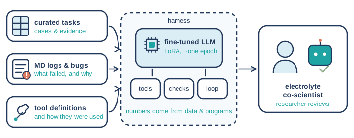
Three kinds of training material
Task records
Formulation and MD cases, reading evidence, a public conductivity dataset (CALiSol), and policy examples: 254,527 rows in the model’s chat and tool format (rows are tasks, not independent formulations).
Logs and bugs
The MD engine’s simulation logs, bugs and failures. The helium incident lives on.
Tools
Tool-usage records plus the tool definitions themselves.
I fine-tuned an open-weight LLM with LoRA for about one epoch, 63,632 steps on one GPU. Fine-tuning teaches the model the task format, how to read evidence, and when and how to call tools. It does not turn the model into a calculator: the numbers still come from the data and the programs.
The harness does the rest
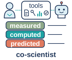 Electrolyte co-scientist
A tool registry (file reading, protocol checks, analysis programs, evidence records, and PFF RSI itself) and a loop: the researcher asks, the LLM plans, and the harness retrieves experiments, calls the explanation and generation models, executes approved simulations, and compares results with saved artifacts.
Deep dive: how a simulation request is handled
Preparing a run is kept separate from submitting it. A request carries the formulation, protocol, resources and a fingerprint, gets validated before a job is ever created, is recognized if it’s a repeat (no burning GPU time on the same run twice), and can recover after a failure. Raw trajectories stay on the tool side; the LLM sees summaries, not 5,000 frames of coordinates.
Three tool fixes I’m proud of
The tools had their own growing pains.
Units
An unsupported unit used to look like “no data,” so the model would conclude nothing existed; now the tool rejects it clearly.
Error messages
With short error messages, the model kept retrying with guessed arguments; now errors spell out the full argument contract.
Identity
One request passed every numeric check while “DMC” was carrying the SMILES of DMF, a different molecule with a confusingly similar name; now the checker verifies chemical identity, which is Part 1’s lesson coming back to collect.
What it can do
It can explain why a simulation failed, how a formulation performed, or how to prepare a run at a new temperature, and the researcher stays in charge by reviewing the next formulations it proposes. This was also when I noticed I was building a way of working more than a single model: represent the liquid, align its views, predict, then hand it to a co-scientist. I’d love to call that a method of my own, but the field moves so fast that I kept adding new pieces to it all summer, so for now it’s a living one.
What this got us
Part 2 gave us a rulebook that covers the molecules people want to try and that learns from its own mistakes, a 128-number description of each liquid learned from recipes, frames and motion, and a co-scientist that knows how to read all of it. Nobody buys a puddle, though. These formulations only matter once they’re sealed inside a real battery, next to electrodes, getting charged and discharged for months, and that’s where Part 3 takes them.